# Forecast
# Overview
The Petro.ai Forecast web application allows for a decline curve analysis workflow featuring batch and single well forecasting as well as a full approvals cycle.
# Petron Forecast Overview
Production forecasting occurs in the Forecast tab. Users can forecast many wells using the Petro.ai Autocasting Engine and then fine tune the resulting decline models with the single well segment editor.
# Batch
When navigating to the FORECAST tab, users will land in batch mode. In this view, users can immediately access settings and forecast desired number of wells. The results and diagnostic information are presented within the same page.
# Single
On the Forecasting tab, users can also select a specific well and drill down into the Single Well Forecast segment editor.
# Forecast Ribbon
The forecast ribbon options are located in the upper right side of the forecast page. This provides the user with options to refresh, perform a single well forecast, change the status of a forecasted well, and run an Auto Forecast.

| Ribbon Options | Description |
|---|---|
| Refresh | Refreshes the tables to their current state. |
| Single Well Forecast | Opens Single Well Forecast application for a selected well. |
| Change Status | Allows the user to submit, unsubmit, reject, approve, or delete selected forecasted wells in the Petron. |
| Auto Forecast | Runs an Auto Forecast for selected wells in the Petron. |
# Forecast Approvals Process
The FORECAST tab contains seven different tables for different stages in the forecasting and approvals process. Each table contains numerous metadata and forecasted value columns allowing the user to filter, sort, and arrange the data in the method of their choosing. Each tab also contains three different interactive views: Table, Probits, and Comparison. This allows the user to quickly analyze and high grade their forecasts.
| Table Names | Description |
|---|---|
| ALL | Contains all wells in Petron |
| NOT STARTED | Contains all wells that do not have a forecast model. |
| AUTO | Contains all wells that have an Auto Forecast model. |
| WORKING | Contains all wells that have a single well forecast adjustment, but has not been submitted for approval yet. |
| REJECTED | Contains wells with a forecast model that have been submitted by an assignee and rejected by the approver. |
| NEEDS REVIEW | Contains wells with a forecast model that have been submitted by an assignee and are awaiting action by the approver. |
| APPROVED | Contains wells with a forecast model that have been submitted by an assignee and approved by the approver. |
# Table
The TABLE icon will display a tabular representation of the data with interactive columns. The user has the option to sort by a column of interest, adjust column position in the table, and add or remove columns from the table. The user can select all wells or a subset of wells and fit decline models on them.
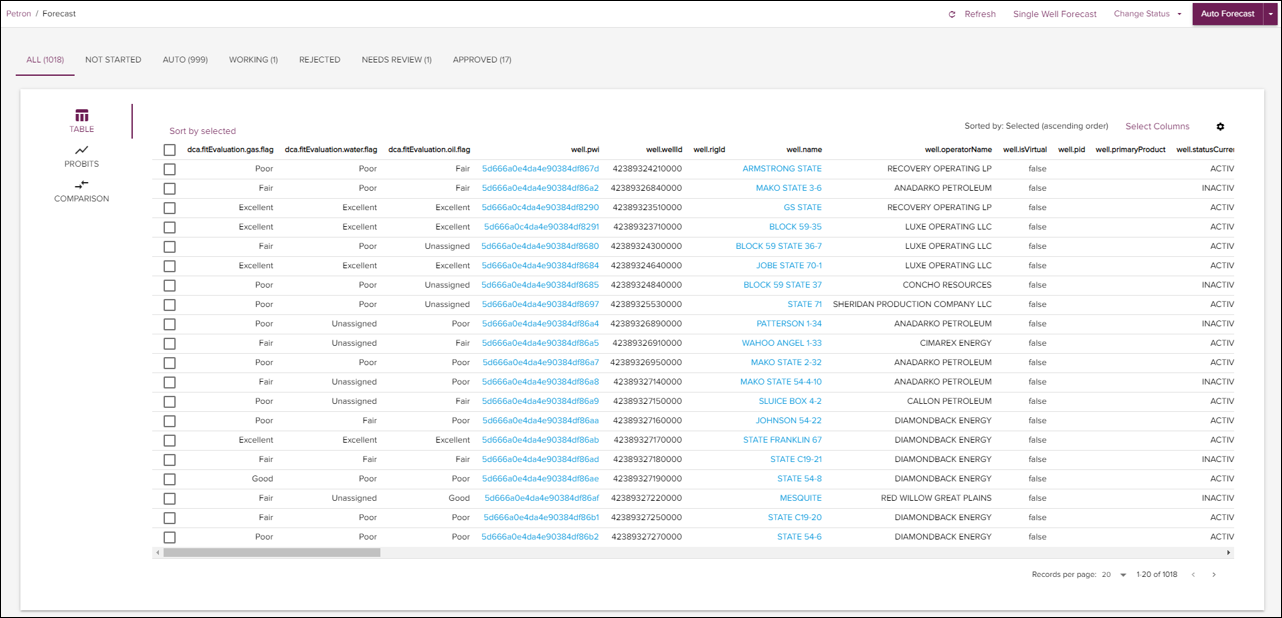
Model Performance
After a batch forecast is executed, model fitness is calculated for each well. Model fitness is determined by comparing the cumulative production to the forecast production over the same time period. This uses the coefficient of determination (R2) to do the comparison. Find the fitness measures below:
| Fitness | Default Threshold |
|---|---|
| Excellent | (<10%) |
| Good | (10-30%) |
| Fair | (30-70%) |
| Poor | (>70%) |
| Unassigned | No flags assigned |
| Insufficient Data | Not enough data points to have a meaningful model |
| Method Failure | Exception thrown while building and training model |
Select Columns
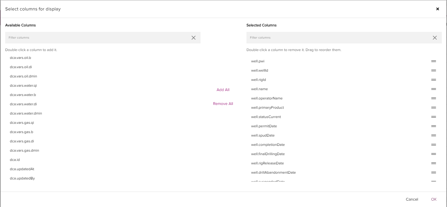
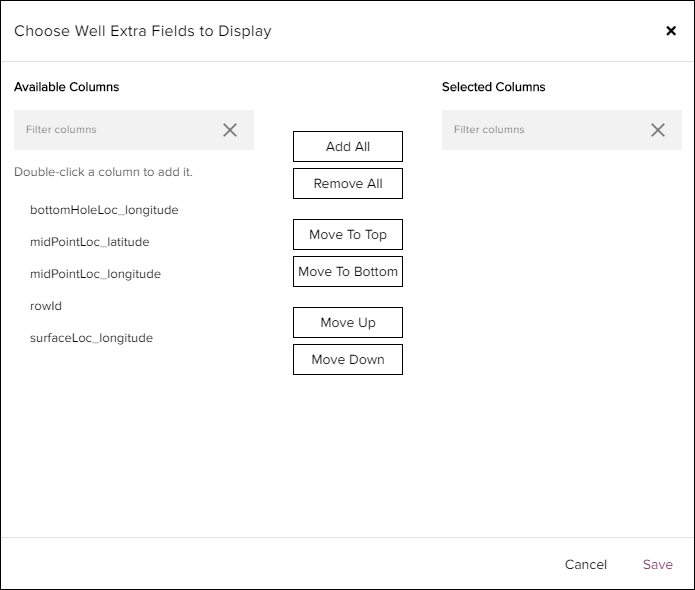
The Select Columns button can be found in the upper right side of the table. Clicking this button opens the select columns menu. The user can look through Available Columns and Selected Columns and add or remove them from the table visual as desired.
There are options to "Add All", "Remove All", "Move To Top", "Move to Bottom" or to double click each individual column of interest. The user can then drag the column to reorder its position in the table.
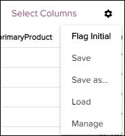
Column Settings
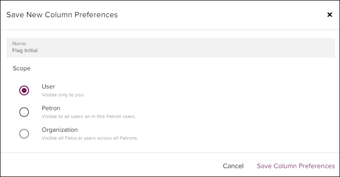
The Column Settings icon allows the user to save, load, or manage the column selection and ordering. A user can save personal column preferences that are visible only to that individual, Petron column preferences visible to all users in this Petron, or Organization column preferences that are visible to all Petro.ai users and across all Petrons.
| Settings Options | Description |
|---|---|
| Save | Save current column preferences (must Save as... prior to enable this option) |
| Save as... | Save current column preferences with new name |
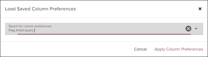
| Load | Load column preferences from a list |
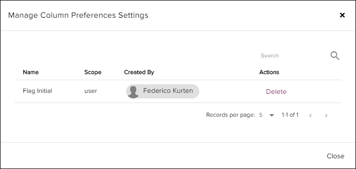
| Manage | Manage list of column preferences, delete |
# Save as
# Load
# Manage
# Probits
Clicking the Probit icon will display a card of probit plots for multiple streams and forecasted decline curve parameters.
A probit plot can help determine if the results trend towards a log-normal or normal distribution. The Y-axis on the probit scale is a non-linear scale that is symmetrical around P50. When combined with the log scale X-Axis, the points of a log-normal distribution trend towards a straight line. The probit chart provides a variety of statistical insight including a measure of uncertainty (P10/P90 ratio).
There are individual probit plot for Oil, Gas, and Water for the following parameters.
| Probit Variables | Description |
|---|---|
| Qi [bbl/d] | Initial Rate of Production. |
| De | Effective Decline Rate. |
| B | Hyperbolic Exponent Factor. |
| Dmin | Limiting decline rate range. Set both numbers as the same value to enforce a hard limit. |
| EUR [bbl] | Estimated Ultimate Recovery |
In addition to the probit plot for those streams, there are BOE6 probit charts for the following parameters.
| Probit Variables | Description |
|---|---|
| EUR [BOE] | Estimated Ultimate Recovery |
| Remaining Reserves [BOE] | Remaining Reserves |
# Using the Probit Plot
The Individual points on the probit plot represent individual forecasted wells, these interactive charts allow the user to select specific ranges of values or single wells based on their position on the probit plot.
- Using the Probit Plot:
Select an indiviual Probit plot of your choice.
Click the range selector icon in the upper right of the plot, (this will highlight once clicked)
Click and drag a range of values on the probit plot. This will highlight those same wells on all other charts respectively.
To remove or undo the selection click the "X" in the upper right side of the plot.
See probit plot workflow below:

# Single Well Forecast
In this section we will discuss the single well forecasting page, where a user can generate an individual decline curve analysis on a well based on the production data.
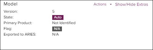
# Model
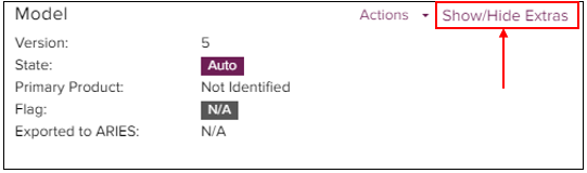
The model area indicates the current version of the forecast model, its current state in the approval process, and whether the model got exported to ARIES.
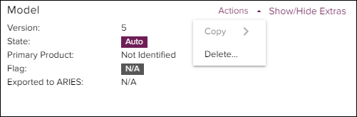
# Actions
The Actions allows the user to delete the current forecast model or copy a compared model onto the current forecast.
# Extras
The Show/Hide Extras allows the user to add or hide any well header fields to the single well forecast page for reference.
# Summary Table
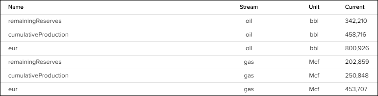
The summary table shows the following metrics and their respective units for a given single well forecast divided per stream. The value under "Current" is updated in real-time as decline parameters change.
| Item | Description |
|---|---|
| RemainingReserves | Estimated recovery from the latest production date through the end of the decline |
| CumProd | Total cumulative production through the latest production date |
| EUR | Estimated ultimate recovery of the well |
# Chart Controls
The main chart on the single well forecast page has a series of controls that are used to toggle and adjust what is being visualized.

# Compare
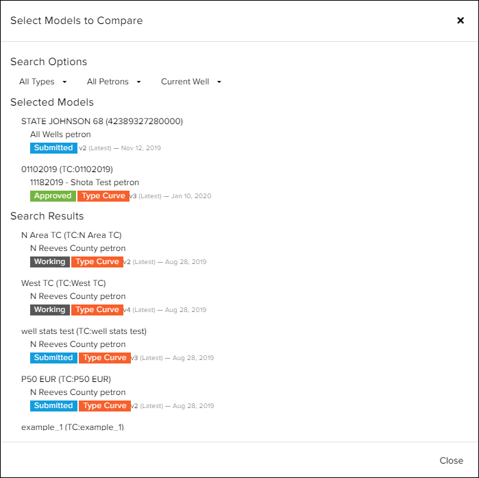
The Compare button allows the user to overlay another forecast model onto the current chart. Adding another model to the current chart also updates the Summary Table. To remove a comparison model, simply click on the name of the model to be removed under "Selected Models."
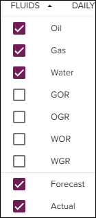
# Fluids Toggle
Use the Fluids Toggle to show or hide any streams that are available for the selected well. The fluid toggle can also be used to hide actual values or forecast curves.
# Vertical Axis Control
The Vertical Axis Control allows the user to select a datatype to visualize on the main chart. The following options are present for the vertical axis:
| Item | Description |
|---|---|
| Daily | Daily production rate and daily production forecast. |
| Monthly | Monthly production rate and monthly production forecast. |
| Cum | Cumulative production and cumulative production forecast. |
| Rate Cum | Daily production rate versus cumulative production. |
# Horizontal Axis Control
The Horizontal Axis Control allows the user to select label options for the horizontal axis.The following options are present for the horizontal axis:
| Item | Description |
|---|---|
| Date | Date of production. |
| Months On | Date of production normalized to month 0, starting from date of initial production. |
# Other Chart Options
The following options on the top right side of the chart are additional features on the single well forecast page.
# Data Download
The Data Download button allows the user to export actual and forecast data into a CSV file.
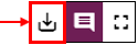
# Comment Toggle
The Comment Toggle allows the user to show or hide the comment lines on the chart.
# Full Screen
The Full Screen button allows the user to maximize the visualization to full screen showing only the chart and the comments.
# Chart Interactions
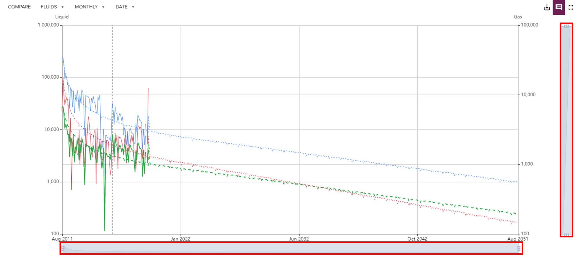
# Axis Zoom Slider
The Axis Zoom Slider can be used to hone in on specific dates and values on the vertical and horizontal axes. The highlighted area is the area selected by the zoom slider.
# Add Comment
To add a comment on the main chart, simply right click on the location where a comment is needed. The Add data comment window will pop up, and the comment can be submitted with the Enter key.
If the Comment Toggle is set to show comments, a dotted vertical line will appear at the location of the comment. To view the text associated with the comment, hover over the dotted line with your cursor.
# Auto Forecast Parameter Edits
The Auto Forecast parameters can be adjusted from the top bar highlighted in the figure below.
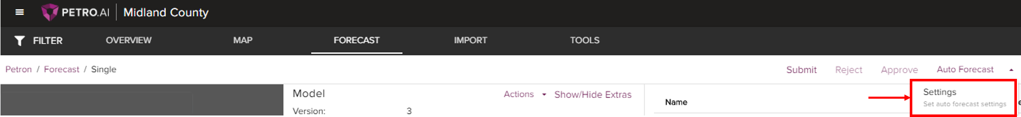
There are multiple methods that can be set up for each stream as well as other non-stream based options that can be configured.
# Stream Based Configuration
| Model | Description |
|---|---|
| Modified Arps | A modified arps hyperbolic decline algorithm will produce the stream's forecast model. See below for parameter adjustment |
| Linear Piecewise | A linear piecewise decline algorithm will produce the stream's forecast model. See below for parameter adjustment. |
| Power Law Exponential | A power law exponential decline algorithm will produce the stream's forecast model. See below for parameter adjustment. |
# Modified Arps Decline Parameters
| Parameter | Description |
|---|---|
| Arps Qi | Range for Initial production rate (Qi). |
| Arps De | Effective Decline Rate. |
| Arps B | Hyperbolic Exponent Factor. |
| Arps Dmin | Limiting decline rate range. Set both numbers as the same value to enforce a hard limit. |
| Zero Threshold | Amount of production rate under which the production is considered as zero. |
| Model Flag Excellent Threshold | Minimum R squared value to consider the model fit excellent. |
| Model Flag Good Threshold | Minimum R squared value to consider the model fit good. |
| Model Flag Fair Threshold | Minimum R squared value to consider the model fit fair. |
TIP
Note: Modified Arps Decline Parameters are adjustable for each stream.
# Linear Piecewise Decline Parameters
| Parameter | Description |
|---|---|
| Scale | Linear or Log10 value scaling. |
| Number of Segments | Number of segments to consider in the continuous Linear Piecewise model. |
| Initial | Initial Rate. If less than or equal to 2, takes the percent of the average rate for the initial period. Otherwise, the absolute rate values are taken into account. |
| Segment Time Days | Range for guessing the length of the linear segment in days (Segment range) |
| Segment Change | Range for guessing the change in slope of the model when switching to the next linear fitting. |
| Outlier SD | Standard deviation (from mean data fit) for declaring points as outliers. |
| Initial Period (days) | Defines the initial period starting from the peak production rate for primary fluid. For example, if 90 is input, the model will begin defining the linear piecewise segments after 90 days. |
| Final Decline | Limiting decline rate (Dmin). The final rate will fit the last segment for the life of the well. |
TIP
Note: Linear Piecewise Decline Parameters are adjustable for each stream.
# Power Law Exponential
| Parameter | Description |
|---|---|
| Power Law Exp Qi | Range for Initial production rate (Qi). |
| Power Law Exp Alpha | Dimensionless parameter derived from loss ratio behavior of unconventional wells ( 1⁄D(t) ). |
| Power Law Exp Beta | Dimensionless parameter derived from loss ratio behavior of unconventional wells ( 1⁄D(t) ). |
| Zero Threshold | Amount of production rate under which the production is considered as zero. |
| Model Flag Excellent Threshold | Minimum R squared value to consider the model fit excellent. |
| Model Flag Good Threshold | Minimum R squared value to consider the model fit good. |
| Model Flag Fair Threshold | Minimum R squared value to consider the model fit fair. |
# Non-Stream Based Configuration
These options are available to set up on a per well basis.
# Forecast Options
| Parameter | Description |
|---|---|
| Years | Number of years to forecast the model. |
| Min. Production Data Points | Minimum number of production data points to create a forecast model. |
| Inactive Decline Date Threshold | Date for which wells with no production after set date will be given an Inactive Decline. |
| Forecast End Date | End date for the forecast model. |
# Normalization
| Parameter | Description |
|---|---|
| Main Fluid | The main fluid to normalize by for a given well. The GOR Threshold parameter is used to determine whether Gas should be considered the main fluid when Main Fluid is set to auto. |
| Date Normalize By | This determines where the normalization for the decline curve should begin. See the Normalization Options below. |
| GOR Threshold | Used to auto-detect the Main Fluid. |
| Type Curve Weight Column | Column Parameter that will be used to normalize type curves. See the Type Curve Weight Column below. Note: Wells with missing values will be removed from the type curve. |
| Target Value | Scale production to this defined value. |
Normalization Options
| Normalization Option | Description |
|---|---|
| Start | The decline curve begins at the start of production history. |
| Local Peak | The decline curve begins at the last local maximum. |
| Global Peak | The decline curve begins at the global maximum production rate. |
| Manual | The decline curve begins at a user defined start date. |
Type Curve Weight Column Options
| Type Curve Weight Column Options | Description |
|---|---|
| Lateral Length | The Lateral Length as the type curve weight |
| Total Proppant | The Total Proppant as the type curve weight |
| Total Fluid Pumped | The Total Fluid Pumped as the type curve weight |
# End of Life [On]
| Parameter | Description |
|---|---|
| Years On | The number of production years to be considered at End of Life. |
| Years End | The number of years to use at the end of life. |
# Limits
| Parameter | Description |
|---|---|
| Gas | Gas cutoff limit. |
| Oil | Oil cutoff limit. |
| Water | Water cutoff limit. |
| OilTTD | OilTTD (cumulative) cutoff limit. |
| GasTTD | GasTTD (cumulative) cutoff limit. |
| WaterTTD | WaterTTD (cumulative) cutoff limit. |
# Forecast Parameter Adjustments
While Auto Forecast parameters can be adjusted, the variables can also be adjusted on the left side panel for each stream. This allows the user to adjust the parameters and visualize the changes in the curve.
# Forecast Settings
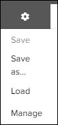
Forecast settings can be saved within the context of the User, Petron, or Environment and loaded later to be applied to other forecasts. To save forecast settings, navigate to the gear on the left ribbon, click "Save As", define the context, and name the forecast settings. To load, navigate to the gear on the left ribbon, click "Load", and select the forecast settings desired.
The "Manage" button allows the user to manage all of the saved forecast settings available in each context.
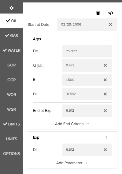
# Fluid Streams
Oil, Gas, and Water all have similar settings in the left ribbon. After an auto forecast, the parameters can be adjusted within the interface to modify the model. Segments can be added or removed.
# The following segment options are available to the user
| Options | Description |
|---|---|
| Modified Arps | A Modified Arps segment |
| Exponential | An exponential decline segment |
| Values | User defined start and end values for a defined duration |
| Flat | Defined flat line production rate |
| Power Law Exponential | A Power Law Exponential segment |
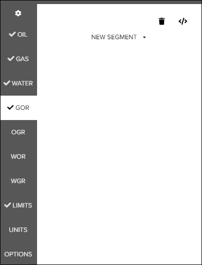
# Ratio Streams
GOR, OGR, WOR, and WGR are available for segment forecasting as well. All of the ratio streams have the same options when setting up declines.
| Options | Description |
|---|---|
| Exponential | An exponential decline segment |
| Values | User defined start and end values for a defined duration |
| Flat | User defined flat line Ratio streams |
# Limits
Limits can be adjusted from the left panel. There are two options to adjust limits:
| Limit | Description |
|---|---|
| Curve Years | Number of years to run the forecast. |
| Volume Abandonment Date | Cutoff date for forecast. Note: If Volume Abandonment Date is manually set, it will be used instead of curve years. |
# Units
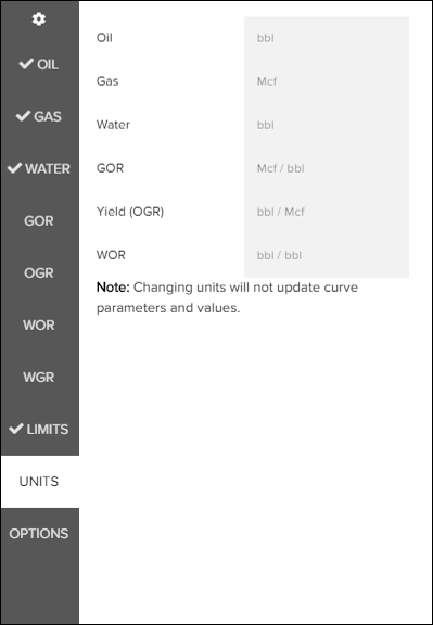
The units tab provides the units' definitions of all streams in the tool.
# Options
The options tab provides the following features:
Flag as Inactive Forecast
# Approval Workflow

Within the Single Well Forecast, the user can submit, approve, or reject the forecast depending on their assignment within a given Petron. The commands will be faded if the user does not have the required permissions as an Assignee or an Approver.
# Well Toggle
On the right side of the top bar, the user can click the arrow keys to navigate to the next marked well in the forecasting table.
# Saving and Comments
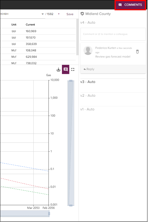
The user can also save a version of the decline model by clicking the "Save" button and later toggle through versions in the Comment section.
Within Comments, the user has a choice to either add comments or toggle through the previous decline versions that were saved. The comments are tied to the single well forecast page and can use searchable hashtags (#) and notification bearing tags (@User).
# Hot Keys
| Keyboard Shortcut | Function |
|---|---|
| Q & W | Previous/Next Well |
| A & S | Increase/Decrease De |
| R & T | Increase/Decrease Qi |
| C & V | Increase/Decrease B |
| N & M | Increase/Decrease Dmin |
| F | Toggles Fluid |
Maps →